
Optimizing for Homogeneity
A population may be composed of distinct subgroups that are subject to different controls or different characteristics and therefore may need to be sampled separately.
To optimize a sample for homogeneity, it is essential to understand how many distinct groups exist in a population. (Of course, the number of groups can vary depending on the definitions of group membership.) A basic analysis using a bar chart can allow auditors to determine the number of distinct groups and the relative size of each group. The idea is to arrive at a manageable number of groups that still allows for a reasonable description of the range that exists in the population; there must also be a plausible rationale for expecting a relationship between the groups and the sampling results. In Figure 7, we show how this could be done by reorganizing the age group data used previously in Figure 2. The data, grouped by strata of 5 years in option 1, can also be presented by strata of 20 years (option 2), thus reducing the number of groups.
The analytical approach used to explore populations and to determine the number of subgroups is often iterative. For example, when analyzing the distribution of a population using a basic histogram, an audit team may need to make half a dozen attempts before it can determine the correct number and width of strata needed to adequately display the distribution of the population. It is worth noting here that the shape of the distribution is a useful indicator of the level of heterogeneity. Normal distributions (i.e., bell-shaped) usually indicate a low level of heterogeneity, while a skewed distribution (often seen when agreements in a population are broken down by value, as in Figure 8) will tend to indicate a high level of heterogeneity. This analysis is important, not only to break a population into meaningful subgroups, but to also to avoid, depending on the purpose of the sampling, creating artificial subgroups.
Once the subgroups are adequately identified, each one should be sampled and tested separately. Each subgroup should be categorized as representing a low, medium, or high risk of deviation or exception (i.e., non-compliance, overpayments, or other, based on the audit objective) and be sampled accordingly. Trying to assess an entire heterogeneous population with a single estimate of a variable under scrutiny will result in a conclusion that does not adequately capture the complexity of the entire population.
In the example in Figure 8, it is assumed that the auditors want to review the contribution agreements awarded by a department for the 2019–20 fiscal year. The funding level varies greatly between agreements. Many have relatively low funding levels (e.g., less than $300,000), while a few have high funding levels (e.g., $1 million to $2 million). How these contribution agreements are managed, and the risk associated with them, likely differs depending on the funding level of each contribution.
In this case, the contribution agreements should be batched into different populations based on funding level. As shown in Figure 8, three subgroups can be identified.
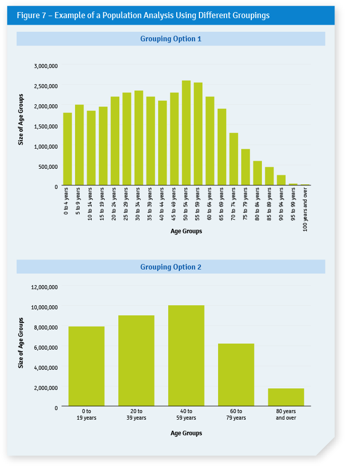
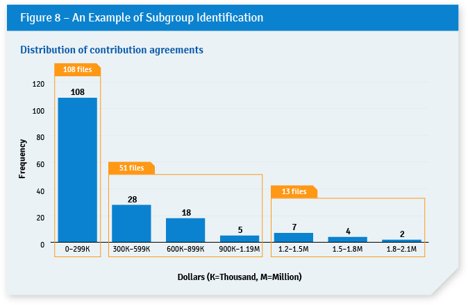
Table 1 provides a more detailed description of the differences among the three subgroups identified in Figure 8, as well as justifications for using different sampling strategies using a risk-based approach.
Table 1 – Comparison of Subgroup Characteristics
|
Subgroups |
Characteristics |
Sampling Strategy |
Comments |
|---|---|---|---|
| Awards with a value between $0–$300,000 | 108 files – Low risk | Small sample | Population is large and risk associated with the files is low. Therefore, a sample with a high level of precision is not needed. (It could also be decided that no assessment is needed at all in light of the low risk level.) |
| Awards with a value between $300,000–$1.2 million | 51 files – Moderate risk | Large sample | Smaller population with moderate risk. A sample with a high level of precision is justified. |
| Awards with a value between $1.2 million–$2.1 million | 13 files – High risk | A sample is not needed—all files are to be examined | Very small population associated with high risks. A census (100% of the files) is warranted because it will provide the highest level of precision. |
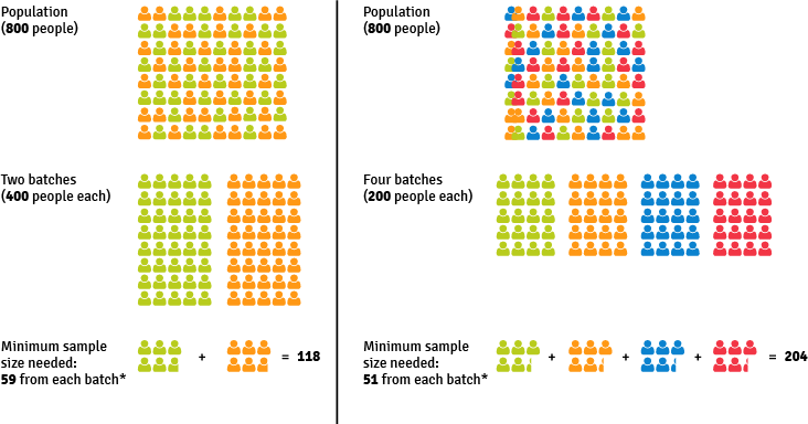
Analyzing the distribution of a population is especially important because the distribution (i.e., how many distinct groups compose the population) has implications for the number of samples that auditors will need to select and has a direct influence on how much time and resources will be required to complete the audit. To minimize the cost of audits, auditors should analyze populations with the goal of creating the smallest number of relatively homogenous subgroups within each population, while taking into account the level of precision required. Table 2 compares two subgrouping strategies, highlighting the advantages and disadvantages of each one.
Table 2 – Example of the Effect of Using Different Numbers of Subgroups for a Survey
*Sample size calculated with confidence interval of 10% and confidence level of 90% using an online sample size calculator.
|
Two Subgroups |
Four Subgroups |
|---|---|
 |
|
| Pros | Pros |
|
|
| Cons | Cons |
|
|
As illustrated in Table 2, having more subgroups implies increasing the costs of conducting a survey for an audit because, overall, more units (members, in this case) need to be selected and examined. This situation involves a trade-off for audit teams between the costs and homogeneity of the samples. Because there are often, in an audit environment, not enough resources to examine more than one or two small samples, the opportunity for auditors to drill down to subgroups may be rare. Therefore, it is incumbent on auditors to assess the level of heterogeneity of the populations before examination.
